Research past 2013: Refer to SDGFEM YouTube channel (link)
[toggle title=”Spacetime Discontinuous Galerkin (SDG) Finite Element method (FEM)” open=”no”][three_fourth last=”no”]
The use of discontinuous basis functions and direct discretization of the spacetime are the two main features of the SDGFEM. Similar to other discontinuous Galerkin methods, SDGFEM has these properties:
- Support for nonconforming meshes and arbitrary basis functions per element; unlike continuous FEMs (CFEMs) no transition elements are needed.
- Per element balance property in discrete setting; CFEMs generally recover balance properties only at the global level.
- Superior performance in handling nonsmooth features compared to CFEMs, particularly for hyperbolic problems.
[/three_fourth][one_fourth last=”yes”]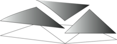
[/one_fourth][three_fourth last=”no”]
The direct discretization of the spacetime using unstructured grids replaces separate time integration and enables:
- Tracking moving interfaces in spacetime.
- Arbitrary resolution in time as the solution is interpolated by spacetime basis functions.
- Elimination of global time increment constraint of time marching schemes.
[/three_fourth][one_fourth last=”yes”]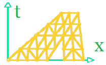 [/one_fourth]
For hyperbolic problems, these two features along with the use of meshes that satisfy special causality constraints provide the following unique features of the SDGFEM:
- Local solution property; each solution stage consists of solving one or a small patch of elements.
- Asynchronous structure as there is no global time step; it is deal for parallel computing.
- Linear complexity in the number of elements. Although many DG methods share this property from the block-diagonal structure of their mass matrices under explicit time integration, it directly stems from the local solution property in the SDG context.
[one_half last=”no”]

Facets of A are “shallower” than the maximum wave speed, so it can be solved once the inflow data is available. Elements 1 can be solved in parallel from initial conditions; elements 2 can be solved from their inflow data and so forth.
[/one_half][one_half last=”yes”]
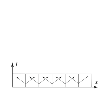
Time marching or the use of extruded meshes imposes a global coupling that is not intrinsic to a hyperbolic problem.
[/one_half][/toggle][toggle title=”Spacetime expression of conservation laws using differential forms” open=”no”]
The spacetime discontinuous Galerkin method requires the expression of balance laws on arbitrary domains in spacetime. Tensorial notation is not appropriate due to the absence of an objective metric in spacetime. We use differential forms to systematically add spatial and temporal quantities. For example, the linear momentum density (conserved quantity) and its spatial flux, stress, are combined to form the spacetime linear momentum flux M. M is a generalization of stress tensor; while traction is the application of a normal vector on stress tensor in space, the restriction of an arbitrary orientation on M delivers the flux in spacetime. The application of the Stokes’ theorem on the balance law yields both the differential equations and jump conditions that are in turn weakly enforced in our SDG formulation. Some other advantages of our approach are:
[one_half last=”no”]
- Revelation of hidden relations in spacetime: Number of independent scales from the dimensional analysis of elastodynamics almost halves in forms compared to tensors.
- Coordinate-free and elegant expressions (e.g. Stokes’ theorem).
- Straightforward derivation of Rankine-Hugoniot (jump) conditions.
- Coordinate transformations: Derivation of various pull-back and push-forward relations in solid mechanics such as Piola–Kirchhoff stresses are much simpler using differential forms’ machinery.[/one_half]
[one_half last=”yes”]
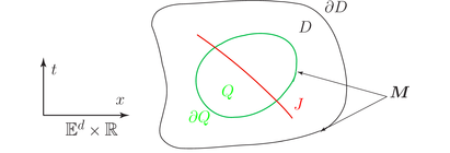
The momentum flux M on arbitrary orientations in spacetime. The differential equation and jump conditions are enforced on Q and J, respectively.
[/one_half][/toggle][toggle title=”Adaptive mesh operations for SDG method” open=”no”]
While the SDG method is already very accurate and efficient due to its local solution and balance properties, exceptional gains are achieved by an hp-adaptive scheme that features:
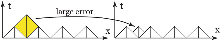
- Local adaptive operations: If error is too large in an element, only that element is rejected; unlike time marching schemes no reanalysis of the entire domain is required.
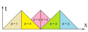
- Arbitrary h-refinement and p-enrichment: Unlike continuous FEMs, the resolution of the mesh and/or element polynomial order can arbitrarily change with no need for special transition elements.
- Arbitrary resolution in time: Due to direct interpolation in spacetime, the solution can locally be resolved with any arbitrary order in time. This is in contrast to time marching schemes where the order of accuracy is often limited by time integration and the same order of accuracy in time is implied for the entire spatial domain.
- No global time increment limit: In explicit time marching schemes the global time step is limited by the smallest elements.

While local time stepping or hybrid implicit-explicit methods (where implicit integration is used for smaller elements)[one_half last=”no”] [/one_half][one_half last=”yes”]
 [/one_half]
remedy this problem to some extent with the added complexity, there is no global time constraint in the SDG method.
This is particularly important in adaptive simulations where element sizes are vastly different. We are currently working on an hp-adaptive version of the SDGFEM.
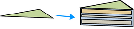
[one_third last=”no”]
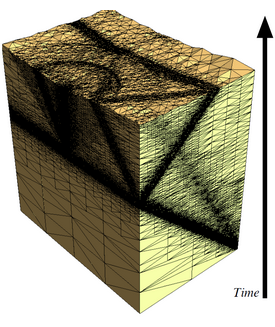
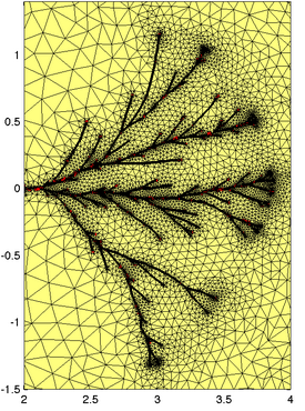
Spacetime mesh of 11 million tetrahedra for a crack-tip wave scattering simulation. The refinement ratio is as small as [latex]10^{-4}[/latex].
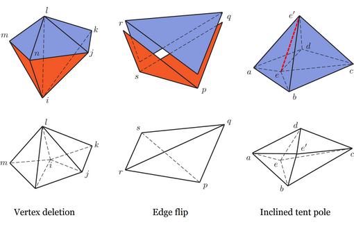
Novel adaptive operations in spacetime (top) facilitate tracking moving boundaries and sharp solution features such as shocks and cracks, without typical projection errors from the old to the new mesh in their spatial counterparts (bottom).
[/two_third][/toggle][toggle title=”Multicell elements: path to a Riemann-free DG method” open=”no”]
In SDGFEM instead of time marching a large coupled system, the solution advances by solving many small patches of elements. This local solution process for hyperbolic problems stems from having causal boundaries on all exterior facets of patches. The elements of a patch, however, are coupled because of noncausal interior facets. Similar to finite volume (FV) and other DG methods, we enforce Riemann fluxes or their numerical approximations on noncausal facets, since they are in accord with the characteristic structure of the underlying hyperbolic problem and are responsible for their inherent accuracy.
The development of a Riemann-free method is a radical advance in computational science as these fluxes are quite cumbersome and expensive to compute, particular for nonlinear and multiphysics problems such as Euler’s fluid equations and Magnetohydrodynamics. The existence of vertical facets implied by time marching nature of other DG and FV methods makes the design of Riemann-free methods almost impossible. However, in SDGFEM all the patch exterior facets are already causal; merging the simplicial cells within a patch to one element eliminates all interior noncausal facets, yielding a Riemann-free method. We have already demonstrated that solving the smaller one-element patches can reduce computational costs for elastodynamics. We plan to solve the Euler’s equations where the elimination of expensive Riemann solutions has even a more pronounced effect.[one_half last=”no”]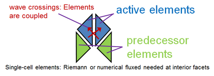 [/one_half][one_half last=”yes”]
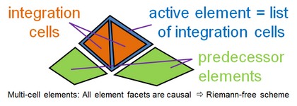 [/one_half][/toggle][toggle title=”Efficient and scalable parabolic solvers” open=”no”]
Many exceptional efficiency and scalability properties of the SDG method rely on the fact that solution cannot propagate faster than the wave speeds implied by the hyperbolicity of a given PDE. For parabolic equations all points of the domain are mathematically coupled; direct discretization of these systems using SDGFEM requires extruded meshes that preserve the global coupling in the discrete setting.
The extension of the local solution and asynchronous properties of the SDGFEM method to parabolic equations is a radical advance in computational science. Besides efficiency improvements, they can eliminate the synchronization constraint of time-stepping methods, a major limiting factor for parallel computing particularly beyond exascale. We have obtained very promising results for uniform meshes by looking at hyperbolic approximations that preserve the method’s inherent order of accuracy. We plan to extend our approach to the more challenging, and yet practical, case of adaptive grids. Our approach can also be applied to hyperbolic systems, such as Magnetohydrodynamics, that possess vastly different wave speeds.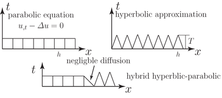
[/toggle][toggle title=”Quantitative comparison of finite element methods” open=”no”]
Although the convergence rates of various numerical methods are known, there is a lack of systematic studies when comparing them in terms of solution cost, effectiveness, memory usage, and performance in parallel environments. In this study we use both analytical and numerical (deal.ii finite element library and the SDGFEM framework) to compare various finite element methods against such measures. A focus of the work is on the scaling and locality of various stages of different methods—such as integration, assembly, and solution—to obtain a better understanding of their performance, particularly in adaptive and parallel settings. Our preliminary comparisons of the SDGFEM method and conventional FEMs with commonly used time integration schemes demonstrate that the SDGFEM method is more efficient even for smooth problems and uniform meshes where some of the advantages of the SDGFEM are not utilized.[/toggle][toggle title=”Dimensional Analysis for dynamic cohesive fracture” open=”no”]
In cohesive fracture models a so-called traction separation relation (TSR), relates tractions to separations on the fracture surface. Accordingly, based on the response for various fracture modes, TSRs are identified with one or a few cohesive stress and displacement scales. To obtain a deep understanding of fracture processes and the interplay of these scales with domain dimensions and various material and load scales, we did a systematic DA for cohesive models. This analysis, the first of its kind, not only yielded the full set of cohesive scales and nondimensional parameters, but also related them to many indicators that were independently proposed before. Examples include brittle-to-ductile transition indicator, maximum time scale for cohesive simulations, and cohesive process zone size.
[/toggle]
[toggle title=”Small Scale Yielding indicator for dynamic fracture” open=”no”]
Linear Elastic Fracture Mechanics (LEFM) models are still widely used in fracture community. These models, however, predict a stress singularity around the crack tip. The small scale yielding (SSY) assumption asserts that LEFM solutions can still accurately represent the overall fracture response, if the size of the region where real material behavior deviates from the singular response is negligible relative to other relevant length scales of the problem. We use more accurate fracture models to characterize the size of this region and identify relevant length scales in dynamic settings to derive universal indicators for SSY indicator. The new indicator determines if the LFEM approach is appropriate for a given dynamic fracture problem.
[one_half last=”no”]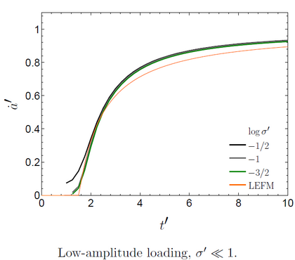 [/one_half][one_half last=”yes”]
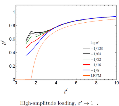 [/one_half]Nondimensional crack speed vs. nondimensional time: As the nondimensional load [latex]\sigma^\prime[/latex]—ratio of applied loads to material strength—increases, crack speed normalized by Raleigh wave speed, [latex]\dot{a}^\prime[/latex], further deviates from that predicted by the LEFM solution, implying the violation of the SSY assumption and loss of accuracy of the LEFM solution.
[/toggle][toggle title=”Quasi-singular velocity response for moving cracks” open=”no”]
Cohesive models, by design, remove the 1/2 nonphysical singularity predicted in the stress field by the Linear Elastic Fracture Mechanics (LEFM) theory. It is not clear whether they eliminate the same singularity that LEFM predicts for velocity fields in dynamic setting. The use of novel cohesive error indicators and extraordinary features of the SDG method enabled exceptional resolutions for the cohesive process zone and led to the discovery of a quasi-singular velocity response.
The LEFM solution implies a region, with radius [latex]r_s[/latex], where the singular velocity field dominates. Within another region of radius [latex]r_p[/latex] velocities vastly deviate from the singular solution and do not tend to infinity. Our theoretical and computational studies demonstrate that, the second region shrinks relative to the singular dominant zone when the crack accelerates, leading to higher velocities. That is, while the velocities are always bounded around the crack tip, they tend to infinity when the crack speed approaches the Rayleigh wave speed. Beyond the theoretical appeal, this phenomenon may help design and calibrate realistic cohesive models.
[one_half last=”no”]
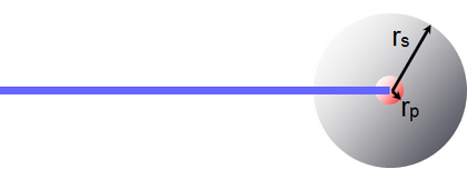
Interaction of the two length scales [latex]r_s[/latex] and [latex]r_p[/latex] is responsible for quasi-singular velocity response.
[/one_half][one_half last=”yes”]
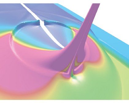
Our very accurate solutions, from the use of SDG method and a secondary error indicator on the fracture surface, led to the discovery of quasi-singular velocity field for cohesive models. Height field: velocity magnitude; Color field: log(strain energy).
[/one_half][/toggle][toggle title=”Multiscale interfacial delay damage model” open=”no”]
According to experiments, high stress fields nucleate small cracks at defects that are randomly distributed in a material. These cracks subsequently advance by processes of void nucleation, growth, and coalescence. In lieu of a traditional cohesive model, we developed a two-scale, interfacial damage model to represent such mesoscopic crack advance processes.
To compare the new model with the more traditional cohesive models we did a dimensional analysis and interestingly obtained identical results for the two. However, unlike cohesive models that are characterized by displacement and stress scales, damage models are determined by a relaxation time scale and a stress scale. This subtle difference mainly stems from the rate-dependent behavior of the damage model and contributes to major differences in their macroscopic behavior, for example in the evolution of fracture process zone and crack propagation history.
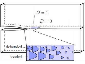
Damage area fraction, D, is determined from a rate-dependent evolution law.
[/toggle][toggle title=”Dynamically consistent contact-damage model” open=”no”]
Rapid contact transitions and sharp moving fronts make dynamic contact modeling very challenging. Numerical solutions are typically marred by prolonged nonphysical oscillations or under/overshoots at these transitions. Artificial diffusion, although may reduce these features, generally overly smoothens the solution. The new set of contact Riemann solutions that we derived preserve the characteristic structure of elastodynamics and enable us to capture these sharp transitions with almost no numerical artifacts. In addition, we integrated these solutions with our interfacial damage model to study combined contact fracture problems.
[one_half last=”no”]
We also investigated the smoothness of various contact mode transitions. For example, the direction of the slip transition is ambiguous at stick-slip transition and it calls for regularization in almost all numerical methods. Using our Riemann solutions, we demonstrate that this transition is in fact continuous and no regularization is required. We show that only separation to contact transition physically induces shocks, for which we propose a regularization scheme with tunable maximum penetration.
[/one_half][one_half last=”yes”]
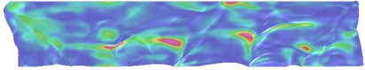
Stick-slip-separation oscillatory waves propagate along the brake/disk contact surface. Height field: velocity; Color field: strain energy.
[/one_half]
[one_half last=”no”]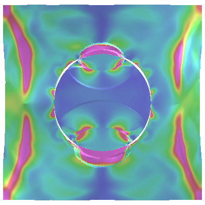 [/one_half][one_half last=”yes”]
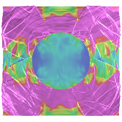 [/one_half]Contact and fracture along the inclusion-matrix interface due to cyclic loading. Fracture initiates at the local debonded site approximately at 1’oclock angle. Height field: velocity; Color field: strain energy.[/toggle][toggle title=”Probabilistic crack propagation” open=”no”][two_third last=”no”]
Stochastic distribution of material defects plays a critical role in fracture processes, particularly in brittle materials. The failure initiated at these weaker sites is often accelerated through increasing stress concentrations induced by initial fracture growth and local inhomogeneity. The energy absorption and stress release through these local features shields surrounding regions and results in a very non-uniform failure pattern at mesoscale.
Deterministic continuum models that treat the material as perfectly homogeneous predict simultaneous failures at regions of high stress, which is not physical. Unfortunately, these problems are somehow shadowed in discrete setting due to slight inhomogeneities implied by numerical errors and often finite loci where cracks can propagate. To address this issue at the continuum level, we devised a probabilistic nucleation model where cracks nucleate from defects that are randomly distributed in the bulk. Our results demonstrate that this representation captures microcracks, crack branching, and cracks surface roughening events and no additional criteria are needed.
To facilitate crack propagation in any arbitrary direction we use the SDG’s powerful adaptive meshing capabilities to align cracks with inter-element boundaries; Unlike X-FEM methods no special discontinuity functions are required.
[/two_third][one_third last=”yes”]
Dynamic crack propagation on the space front. Refinement ratio is smaller than [latex]10^{-6}[/latex].
[/one_third][/toggle][toggle title=”Structural Health Monitoring for composite laminates” open=”no”]
 The development of a flexible, accurate, and efficient computational framework for composite laminates can be challenging. The low -order in-thickness 2D idealizations produce stiff solutions with larger than an order of magnitude error in deflections for thick plates. Higher-order models are difficult to formulate and the governing equation change based on in-thickness kinematic assumption, making their implementation cumbersome. We developed a combined 2D-3D approach within the SDG framework where the domain is discretized as a 2D object, but arbitrary in-thickness kinematics are directly integrated during solution. This approach combines the simplicity of 2D discretization with the accuracy and flexibility of 3D models. It also permits abrupt or gradual changes to laminate configuration and layer thicknesses. We are currently incorporating various failure models for the structural health monitoring of these structures.
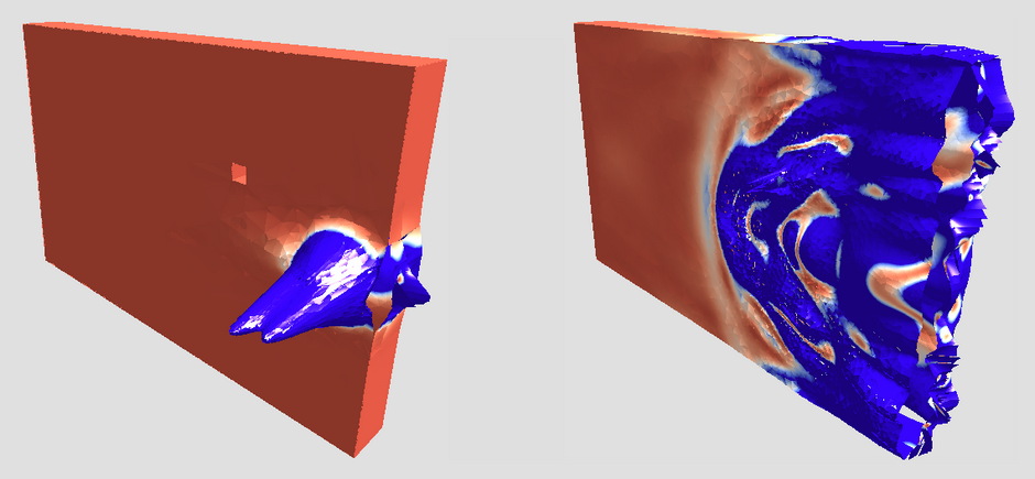
The study of wave scattering off of a hole from a sinusoidal impulse load in a 2-ply composite plate. Height field: velocity; Color field: strain velocity.
[/toggle]